Sponsors


Scipy Tutorial
Scipy:
First let's import the Scipy library with the following command:
In [1]: import scipyDefine the polynomial (2*x ^2 +5*x+7):
In [2]:p = scipy.poly1d([2, 5, 7])

In [3]:p
Out[3]: poly1d([2, 5, 7])
In [4]:print p
2
2 x + 5 x + 7In [5]: x = np.linspace(-10, 10, 21)
In [6]:plt.plot(p(x))
Out[6]: [<matplotlib.lines.Line2D at 0x23750470>]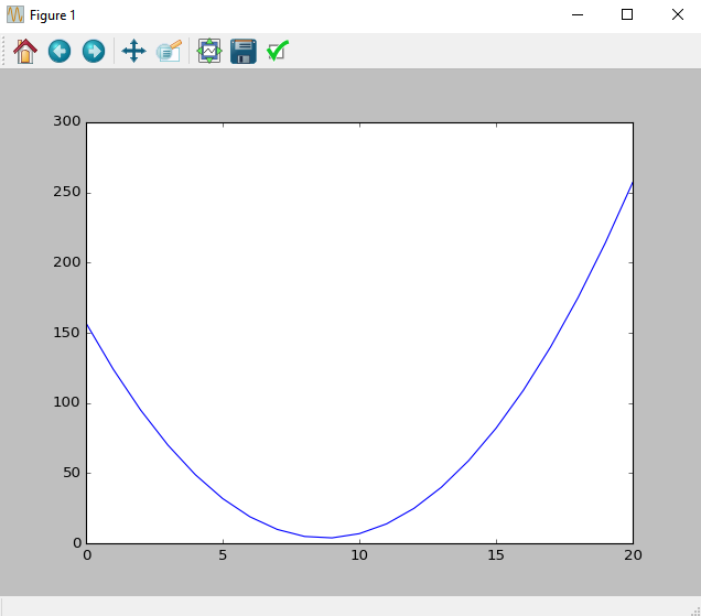
Now we will import the library linalg of Scipy. This library will allow us to perform various mathematical operations on arrays. We'll start with actions on matrixes:
Note that a similar library can be imported from the library numpy, but the one that in scipy is faster and more recommended.
In [6]: from scipy import linalgMatrix multiplication:
Notice that if we'll multiply two-dimensional arrays (matrices) a simple multiplication. we'll get a new vector in which each organ is the product of two elements in the same place respectively at matrices A, B. Lets preform some example:
In [7]: A = np.full((3, 3), 3, dtype=int)

A
Out[7]:
array([[3, 3, 3],
       [3, 3, 3],
       [3, 3, 3]])

In [8]: B=np.arange(9).reshape(3,3)

B
Out[8]:
array([[0, 1, 2],
       [3, 4, 5],
       [6, 7, 8]])

In [9]: A*B
Out[9]:
array([[ 0,  3,  6],
       [ 9, 12, 15],
       [18, 21, 24]])
In order to perform a valid matrix multiplication we use the following command:
In [10]: A.dot(B)
Out[10]:
array([[27, 36, 45],
       [27, 36, 45],
       [27, 36, 45]])
Matrix Transpose:
In [11]: B.T
Out[11]:
array([[0, 3, 6],
       [1, 4, 7],
       [2, 5, 8]])
Inverse:
In [12]: I = np.array([[1, 2, 3],
                       [0, 5, 6],
                       [0, 0, 9]])

In [13]: linalg.inv(I)

Out[13]:
array([[ 1.        , -0.4       , -0.06666667],
       [ 0.        ,  0.2       , -0.13333333],
       [ 0.        ,  0.        ,  0.11111111]])
Determinant:
In [14]: C = np.array([[1, 2, 3],
                       [7, 8, 6],
                       [4, 5, 6]])

In [15]: linalg.det(C)
Out[15]: -8.999999999999998
Norm:
In [16]: C = np.array([[1, 2, 3],
                       [1, 4, 9],
                       [1, 16, 81]])
norm 1, frobenius, infinity :
In [17]: linalg.norm(C, 1)----> Norm 1(The organs maximum sum at columns)
Out[17]: 93.0

In [18]: linalg.norm(C, 'fro')---->  Frobenius norm(Root sum of the squares of all  organs)
Out[18]: 83.246621553069645

In [19]: linalg.norm(C, np.inf)----> Infinity norm(The organs maximum sum at raws)
Out[19]: 98.0
interpolate :
We will import interp1d class which allows to perform interpolation on a one-dimensional arrays.
In [20]: from scipy.interpolate import interp1d
In [21]: x = np.linspace(0, 10,11)

In [22]: y = np.cos(x)

In [23]: plt.plot(x,y)
Out[23]: [<matplotlib.lines.Line2D at 0x2c843cc0>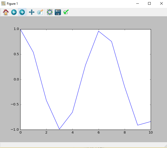
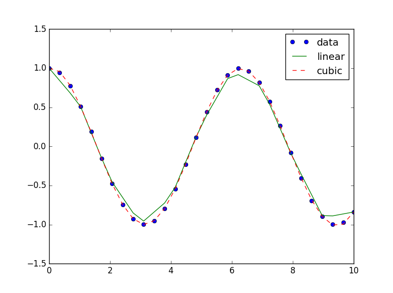
For example, we will use two types of interpolations. First, a linear interpolation. And second, finer interpolation and more accurate one('cubic').
For this example, we created a new vector which divided into more intermediate values.
In [24]: x
Out[24]: array([  0.,   1.,   2.,   3.,   4.,   5.,   6.,   7.,   8.,   9.,  10.])
In [25]: x2 = np.linspace(0, 10,30)
y = np.cos(x)
I1 = interp1d(x, y)
I2 = interp1d(x, y, 'cubic')
I1,I2 behave like functions. We created I1,I2 accordind to vector x and we activate it on vector x2 which is finer. the function will returns us to the values of y by interpolation according to the vercotr x:
In [26]: plt.plot(x2, np.cos(x2), 'o', x2, I1(x2), '-', x2, I2(x2), '--')
         plt.legend(['data', 'linear', 'cubic'], loc='best')
Note that ("loc='best') Placing the legend in the most optimal place. for hiding less information from the graph as possible.
scipy.stats:
This directory contains many statistical functions. They all operate under the same
Principles of the normal distribution:
First we need to import the following libraries:
In [1]: import numpy as np

In [2]: import matplotlib.pyplot as plt

In [3]: from scipy import stats

In [4]: %matplotlib
Using matplotlib backend: Qt4Agg
We will create a normal distribution (Expected value 0.25,standard deviation 1) by use the following commands:
In [5]: x = np.linspace(-5, 5, 150)

In [6]: n = stats.norm(0.25, 1)

In [7]: plt.plot(x, n.pdf(x),lw='3')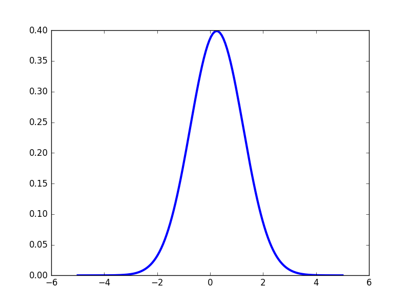
Histogram:
We will use n.rvs function to creates 50 (An arbitrary number) random values at chosen distribution. In our case a normal distribution. The histogram divided into ten bins:
In [69]: n = stats.norm()
         x = n.rvs(50)
         h = stats.histogram(x, numbins=10)
plt.bar(range(h[0].size), h[0], color='green') 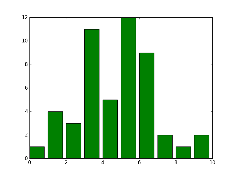
Recent Stories


Top DiscoverSDK Experts


Featured Products


Compare Products
Select up to three two products to compare by clicking on the compare icon () of each product.
{{compareToolModel.Error}}
{{CommentsModel.TotalCount}} Comments
Your Comment