NumPy Advanced Topics

In this article, we’ll continue with what we covered in Getting started with NumPy and will take a look at some more advanced features.

Again, my idea behind these articles is to give a deeper understanding on Data Science with Python by learning the basics. Let's continue and see what more can we do with NumPy.

Dots

Last time I missed one part of slicing NumPy arrays, dots. We have seen that we can slice dimensions which are not required with the colon symbol (:) and if we need the last dimension, we can omit the colon:

>>> a = np.arange(10, 40).reshape(3,5,2)
>>> a
array([[[10, 11],
       [12, 13],
       [14, 15],
       [16, 17],
       [18, 19]],

      [[20, 21],
       [22, 23],
       [24, 25],
       [26, 27],
       [28, 29]],

      [[30, 31],
       [32, 33],
       [34, 35],
       [36, 37],
       [38, 39]]])
>>> a[:, 1, :]
array([[12, 13],
      [22, 23],
      [32, 33]])
>>> a[:, 1]
array([[12, 13],
      [22, 23],
      [32, 33]])

Now using dots (...) we can represent as many dimensions as needed to produce the complete indexing tuple:

>>> a[:, :, 1]
array([[11, 13, 15, 17, 19],
      [21, 23, 25, 27, 29],
      [31, 33, 35, 37, 39]])
>>> a[...,1]
array([[11, 13, 15, 17, 19],
      [21, 23, 25, 27, 29],
      [31, 33, 35, 37, 39]])

For small dimensions this does not make a difference but if you have larger dimensions, you have to type less to get the data you need.

Indexing with boolean arrays

Indexing is done normally through numbers, the index. NumPy goes a step further and enables indexing through boolean arrays. The trick behind this is that such arrays work as a filter. We define a boolean array to tell NumPy which numbers we need (True) and which we don't (False):

>>> a = np.arange(10, 40).reshape(5,6)
>>> a
array([[10, 11, 12, 13, 14, 15],
      [16, 17, 18, 19, 20, 21],
      [22, 23, 24, 25, 26, 27],
      [28, 29, 30, 31, 32, 33],
      [34, 35, 36, 37, 38, 39]])
>>> idx = np.array([[True, False, True, False, True, False],
                   [True, False, True, False, True, False],
                   [True, False, True, False, True, False],
                   [True, False, True, False, True, False],
                   [True, False, True, False, True, False]
                 ], dtype=bool)
>>> a[idx]
array([10, 12, 14, 16, 18, 20, 22, 24, 26, 28, 30, 32, 34, 36, 38])

In the example above we have created a NumPy array which contains boolean values. Now if we provide this as an indexing parameter to another NumPy array (which has the same dimensions) we filter out the values to a vector (1 dimensional matrix) where the index contains True.

We can provide an slightly differently shaped array for indexing too, but then you will get a warning:

>>> idx = np.array([[True, False, True, False, True, False],
                   [True, False, True, False, True, False],
                   [True, False, True, False, True, False]
                 ], dtype=bool)
>>> a[idx]
__main__:1: VisibleDeprecationWarning: boolean index did not match indexed array along dimension 0; dimension is 5 but corresponding boolean dimension is 3
array([10, 12, 14, 16, 18, 20, 22, 24, 26])

The warning tells us that we provided a wrong-shaped array for the index—but we get back all the values we want to get, NumPy interprets the missing dimensions as completely filled with False.

And based on this knowledge we can go a step further and we can filter values, not only by manually generating boolean arrays to filter but let NumPy do the creation:

>>> idx = a > 25
>>> idx
array([[False, False, False, False, False, False],
      [False, False, False, False, False, False],
      [False, False, False, False,  True,  True],
      [ True,  True,  True,  True,  True,  True],
      [ True,  True,  True,  True,  True,  True]], dtype=bool)
>>> a[idx]
array([26, 27, 28, 29, 30, 31, 32, 33, 34, 35, 36, 37, 38, 39])

In this example we let NumPy create a boolean array and we filtered out the values which are greater than 25.

Loading mixed content

We have seen in the previous section that we can create arrays of non-numeric types (like boolean). Now it is time to use this knowledge and load a CSV file with mixed content.

For this we will use a dataset about the Most Popular Baby Names by Sex and Mother's Ethnic Group, New York City. I have downloaded the CSV version and named it baby_names.csv, so you can follow along and try the examples yourself on the dataset.

The file has the following header:

BRTH_YR,GNDR,ETHCTY,NM,CNT,RNK

To write it down to a readable format:

1. Birth Year
2. Gender
3. Ethnicity
4. Name
5. Count
6. Rank

Let's start by loading the file with NumPy as we have learned in the previous article:

>>> baby_names = np.genfromtxt('baby_names.csv', skip_header=True, delimiter=",")
>>> baby_names
array([[ 2011.,    nan,    nan,    nan,    13.,    75.],
      [ 2011.,    nan,    nan,    nan,    21.,    67.],
      [ 2011.,    nan,    nan,    nan,    49.,    42.],
      ...,
      [ 2014.,    nan,    nan,    nan,    16.,    96.],
      [ 2014.,    nan,    nan,    nan,    90.,    39.],
      [ 2014.,    nan,    nan,    nan,    49.,    65.]])
>>> baby_names.shape
(13962, 6)

The example shows you what happens if we use the default datatype for NumPy arrays, float: you get a lot of nan-s which means not a number. And this is right—the dataset consists of a lot of string information which cannot be converted to float.

Now let's go a step further and load the information in the right format.

>>> baby_names = np.genfromtxt('baby_names.csv', skip_header=True, delimiter=",", dtype='U75')
>>> baby_names
array([['2011', 'FEMALE', 'HISPANIC', 'GERALDINE', '13', '75'],
      ['2011', 'FEMALE', 'HISPANIC', 'GIA', '21', '67'],
      ['2011', 'FEMALE', 'HISPANIC', 'GIANNA', '49', '42'],
      ...,
      ['2014', 'MALE', 'WHITE NON HISPANIC', 'Yusuf', '16', '96'],
      ['2014', 'MALE', 'WHITE NON HISPANIC', 'Zachary', '90', '39'],
      ['2014', 'MALE', 'WHITE NON HISPANIC', 'Zev', '49', '65']],
     dtype='<U75')

The difference is that I have added the dtype argument to the genfromtxt function. The value U75 specifies that we want to read every value as a 75 byte unicode.

The skip_header argument specifies that we want to skip the header, which is the first row of the CSV file.

The drawback of this approach is that you get every column as a string, even the numeric ones. This is because NumPy requires that every element is from the same type so it does not need to check types every time—this makes it fast while dealing with a lot of data.

Naturally there is a solution if you want to convert a column to a number because you want to do some calculations on it. For example let's calculate the male and female baby names in 2011:

>>> year_filter = baby_names[:,0] == '2011'
>>> female_filter = baby_names[:,1] == 'FEMALE'
>>> male_filter = baby_names[:,1] == 'MALE'
>>> male_2011 = year_filter & male_filter
>>> female_2011 = year_filter & female_filter
>>> baby_names[female_2011]
array([['2011', 'FEMALE', 'HISPANIC', 'GERALDINE', '13', '75'],
      ['2011', 'FEMALE', 'HISPANIC', 'GIA', '21', '67'],
      ['2011', 'FEMALE', 'HISPANIC', 'GIANNA', '49', '42'],
      ...,
      ['2011', 'FEMALE', 'WHITE NON HISPANIC', 'ZISSY', '25', '66'],
      ['2011', 'FEMALE', 'WHITE NON HISPANIC', 'ZOE', '81', '28'],
      ['2011', 'FEMALE', 'WHITE NON HISPANIC', 'ZOEY', '21', '70']],
     dtype='<U75')
>>>
>>> female_count =  np.sum(baby_names[(female_2011), -2].astype(int))
>>> male_count =  np.sum(baby_names[(male_2011), -2].astype(int))
>>> female_count
117948
>>> male_count
153748
>>> np.sum(baby_names[(year_filter), -2].astype(int))
271696
>>> female_count+male_count
271696

As you can see, I have created some filters which can be used later on with the base array to select only those values we are interested in. I split up the filters into basic parts (year_filter, female_filter, male_filter) and then combined them together into the final ones (female_2011, male_2011).

The selection baby_names[(female_2011), -2] selects all the lines containing female names from the dataset and gets only the second to last column, which is the count of these names. After this is selected, we can convert the values in this vector (the selected column) to an integer with the .astype(int) method call. Finally we sum-up the numbers.

Finally, I have created a verification too to see that we selected the right values and do not have any entries in our dataset where the gender is missing.

Views and copies

Now we have arrived at a topic which can be confusing for the beginning NumPy user: When is an array copied? Let's see a basic example with Python:

>>> a = [1,2,3,4,5,6]
>>> b = a
>>> a is b
True
>>> b[2] = 11
>>> a
[1, 2, 11, 4, 5, 6]

And now the same with NumPy:

>>> import numpy as np
>>> a = np.array([1,2,3,4,5,6])
>>> b = a
>>> a is b
True
>>> a.shape
(6,)
>>> b.shape = 3,2
>>> a
array([[1, 2],
      [3, 4],
      [5, 6]])

As you can see, when we assigned the value of a to b we did not create a copy but passed the reference to the original contents to the new variable. If we change something in the new variable it is reflected on the original variable too, for example changing the shape or the contents.

You can achieve a different behavior with views on the original array:

>>> import numpy as np
>>> a = np.array([1,2,3,4,5,6])
>>> b = a.view()
>>> b
array([1, 2, 3, 4, 5, 6])
>>> b.shape = 2,3
>>> b
array([[1, 2, 3],
      [4, 5, 6]])
>>> a
array([1, 2, 3, 4, 5, 6])

But beware: using the view() method on arrays creates a copy which references the elements of the original array; changing the shape has no effect on the original but changing the values does:

>>> b[0, 2]
3
>>> b[0, 2] = 12
>>> a
array([ 1,  2, 12,  4,  5,  6])
>>> b.flags.owndata
False
>>> b.base is a
True

If you look at the code snippet above you can see that changing a value in b changes the value in a too, even if they have different shapes. The reason can be seen in the owndata flag of the new array—it does not have its own data, it shares the data of the original.

If you want really a copy which does not share the variables, you can do this too:

>>> a
array([ 1,  2, 12,  4,  5,  6])
>>> b = a.copy()
>>> b.base is a
False
>>> b.flags.owndata
True
>>> b.shape = 2,3
>>> b[0,0] = 11
>>> a
array([ 1,  2, 12,  4,  5,  6])
>>> b
array([[11,  2, 12],
      [ 4,  5,  6]])

Now we have a really independent new array which was based on the state of a at the time when calling copy() and there is no more a relation between the two variables.

Arithmetic

If you apply an arithmetic operation on a NumPy array, it will be applied on all the elements, and a new array is created with the results.

Actually there is not much to talk about with this topic; we will simply use basic arithmetic operators:

>>> import numpy as np
>>> a = np.array([1,2,3,4,5,6])
>>> a + 4
array([ 5,  6,  7,  8,  9, 10])
>>> array * 5
array([ 5, 10, 15, 20, 25, 30])
>>> a - 10
array([-9, -8, -7, -6, -5, -4])
>>> a / 2
array([ 0.5,  1. ,  1.5,  2. ,  2.5,  3. ])
>>> a // 2
array([0, 1, 1, 2, 2, 3])

If we use the in-place version of these operators, we get the same results: the array is modified in-place and the operation is done on all the elements of the array:

>>> a = np.array([1,2,3,4,5,6])
>>> a += 4
>>> a
array([ 5,  6,  7,  8,  9, 10])
>>> a *= 5
>>> a
array([25, 30, 35, 40, 45, 50])
>>> a -= 10
>>> a
array([15, 20, 25, 30, 35, 40])
>>> a //= 2
>>> a
array([ 7, 10, 12, 15, 17, 20])
>>> a = np.array([ 7, 10, 12, 15, 17, 20], dtype=float)
>>> a
array([  7.,  10.,  12.,  15.,  17.,  20.])
>>> a /= 2
>>> a
array([  3.5,   5. ,   6. ,   7.5,   8.5,  10. ])

As you can see, to use the in-place division operator (/=) you have to convert the array to a dtype capable of handling floating point numbers.

However there are certain functions in NumPy which convert matrices of integer elements to floating point matrices:

>>> a = np.array([ 7, 10, 12, 15, 17, 20])
>>> a.dtype
dtype('int64')
>>> np.sin(a)
array([ 0.6569866 , -0.54402111, -0.53657292,  0.65028784, -0.96139749,
       0.91294525])
>>> np.sin(a).dtype
dtype('float64')

Plotting histograms

OK, this topic is not really part of NumPy because you need an extra library but after these introductory articles I’ll also give you an example where NumPy plays along with other tools.

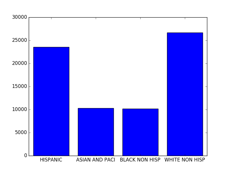
However, this article is not about plotting. Therefore we will just create a simple plot based on the baby names information used in this article We will plot the count of names in 2012 split by ethnicity.

>>> year_2012 = baby_names[:, 0] == '2012'
>>> ethnicities = np.unique(baby_names[(year_2012), 2])
>>> for e in ethnicities:
...     ethnicity_filter = baby_names[:,2] == e
...     sums[e] = np.sum(baby_names[(year_2012 & ethnicity_filter), -2].astype(int))
...
>>> sums
{'HISPANIC': 23547, 'ASIAN AND PACI': 10300, 'BLACK NON HISP': 10208, 'WHITE NON HISP': 26675}

As you can see, we stored the results in the sums dictionary to have a relation between the ethnicities and their numbers.

This is one approach, you can do it differently as well. For example, filter out the whole dataset right at the beginning and use only the rows containing 2012 data later on (like when we calculated the unique ethnicities).

>>> import matplotlib.pyplot as plt
>>> plt.bar(range(len(sums)), sums.values(), align='center')
>>> plt.xticks(range(len(sums)), sums.keys())
>>> plt.show()

The last part is the plotting itself. We create a bar chart using matplotlib, the height of each bar is defined by the count of the given ethnicity (the values of the sums dictionary).

And the result is something like this:

Conclusion

We have finished the introduction into NumPy with some advanced topics. We have seen that the performance of NumPy is best if we have all data of the same type, meaning that sometime we have numeric columns as strings in our matrix.

Next time we will continue our data science introduction with Pandas where we will take a deeper look on data frames and what's behind the idea.